Creating a Listserv to use with your Canvas course
Estimated Reading Time: 3 MinutesNote: prior to 2025, a Listserv was automatically created with each Canvas course. Starting in January of 2025, if you want a Listserv for your course, you will need to create it manually. Here are the instructions to do that using Excel. You will need a little Excel experience to do this. Please note that there are a lot of ways to do this - the important thing is to get the usernames with a comma after them and Copy them - then Paste them into Central. If you have a small group you can also just type them in.
START IN CANVAS
Open your Canvas course.
Go to Grades for the Gradebook.
Click on Export and select Export Entire Gradebook. It will download into your Downloads folder as a .CSV file that you can open in Excel.
USE EXCEL TO GET THE USERNAMES IN THE RIGHT FORMAT
Once you open it, you will see the second row "Points Possible". Let's start by deleting this row (Row 2). Now the column names will be in Row 1, and the student information will start in Row 2. (Optional)
Notice that column D has the email address which is the UserName followed by @clemson.edu. What we need is the username followed by a comma.
We don't need the columns after D - so we'll just overwrite them as we need a new column. In the end we will not be saving the file - just highlighting the cells in the right format, copying, then pasting into Central.
Highlight Column E and and press the Delete key on your keyboard to erase the contents (don't delete the column, just make it blank). Rename the column title on Row 1 to Characters in UserName (optional - just to help us keep this straight).
Go to Cell E2. Type in FIND("@",D2,1)-1 as the formula for that cell. When you press enter, you will see the number of characters in the username. This formula, Find, finds the position of the "@"in the email address in cell D2. We subtract 1 from it to get the number of characters in the UserName. The username wxbrahm has 7 characters.
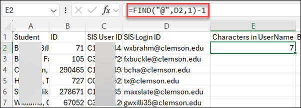
Now copy Cell E2 and Paste it into all of the cells below it (for all of the students). Once you paste, you should see a one digit number representing the number of characters in each user name.

Select Column F. Erase the contents of the cells in the column pressing the Delete key on your keyboard. Name the column title to UserName (optional - just to keep this straight).
Go to Cell F2. Type in LEFT(D2,E2)&"," as the formula for that cell. When you press enter, you will see the student's username with a , after it.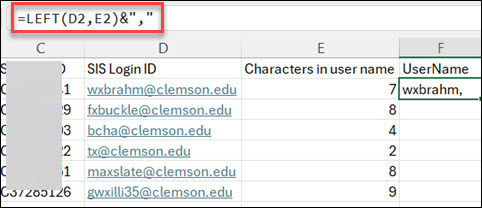
Copy Cell F2 and Paste to all of the cells beneath it that are next to student names.
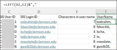
One more step. The username cells are now actually formulas. But we need them to be in text format. So go to Column G. Rename the column title to UserName Text (optional - just to keep this straight) and erase any content from cells under it.
Now highlight all of the cells in Column F (except the column title). Right-click and select Copy.
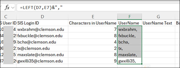
Go to Cell G2, right-click, under Paste Special select Paste Values.
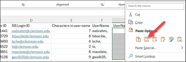
If you highlight any of the cells you should see the username with , and not the formula.
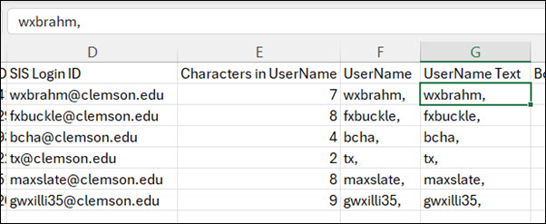
To get it into the Central group so you can create a ListServ, highlight all of the cells under Column G (not including the title), and select Copy.
GO TO CENTRAL
Open a browser window and go to https://central.clemson.edu
Click on + CREATE to create a new Central Group giving it a name.
Click on the Pencil/Edit button to edit the settings for the group.
Click on USERS and Batch Edit.
Paste the students under Members and click Submit.
Go to Settings and turn lists.clemson.edu on with the slider and then click Save.
If you have more questions, email ITHELP@clemson.edu or call 864-656-3494.